Reproducing a Deep Learning Paper

By Asror Wali - 4981081 - a.wali-1@student.tudelft.nl

& Erwin Russel - 4973976 - e.f.j.russel@student.tudelft.nl

This is a short blog about a reproduction of the paper “W-Net: A Deep Model for Fully Unsupervised Image Segmentation”. This reproduction is part of the CS4240 Deep Learning course at the TU Delft.

We were asked to choose from a list of papers, where this was the one we found most interesting. There was a Github repository attached to the paper which we could use, in this blog we will describe the process of using this code repository and adapting it to achieve the results that were displayed in the paper. Next to reproducing the cool segmentation abilities of the WNet architecture, we also want to see how our reproduction benchmarked against the model in the paper. There is a table explaining various benchmarks that we will go into in this blog.

The dataset is discussed following the losses and postprocessing. We are showing preliminary results on a small dataset, since the original paper trained the model 50000 epochs on 12000 images this was not attainable given the resources given (google cloud and educational credit). We therefore show one of the results training on a miniscule dataset size of only 10 images running with 100 epochs.

Reproduction is a very important task in the field of Deep Learning, and as it turns out, reproduction is HARD. Missing data, code, specifications and more is common in Deep Learning research papers. And while said research can be groundbreaking, it is of no use when it cannot be replicated. We tried to be as thorough as possible in our reproduction but must state that given the time and budget of our reproduction it can be seen as an attempt to reenact this research and documenting our findings along the way. If there are any questions about this blog or the Github repository, please feel free to contact us at our emails (Asror or Erwin) or opening a Github issue.

Dataset

W-Net uses two different datasets, they train the network using the PASCAL VOC2012 dataset and evaluate the network using the Berkeley Segmentation Database (BSDS 300 and BSDS 500). The PASCAL VOC2012 dataset is a large visual object classes challenge which contains 11,530 images and 6,929 segmentations. BSDS300 and BSDS500 have 300 and 500 images including human-annotated segmentations ground truth. The images are divided into a training set of 200 images, and a test set of 100 images. The ground truth are Matlab files that are 2D matrices with the annotated labels, with multiple segmentations. The different segmentations for a single picture can be seen below.

The Model

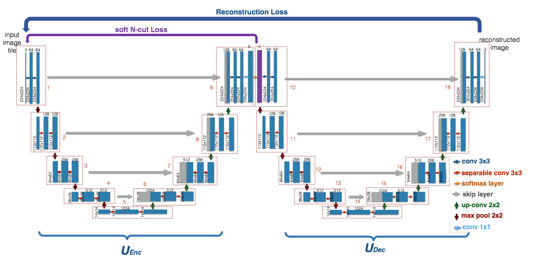
The W-Net model consists of 2 U-Nets, the first U-Net works as an encoder that generates a segmentated output for an input image X. The second U-Net uses this segmentated output to reconstruct the original input image X.

To optimize these 2 U-Nets, the paper introduces 2 loss functions. First, A Soft Normalized Cut Loss(soft_n_cut_loss), to optimize the encoder and Secondly a Reconstruction Loss(rec_loss), to optimize both the encoder and the decoder.

The soft_n_cut_loss simultaneously minimizes the total normalized disassociation between the groups and maximize the total normalized association within the groups. In other words, the similarity between pixels inside of the same group/segment gets maximized while the similarity between different groups/segments get minimized.

The rec_loss forces the encoder to generate segmentations that contain as much information of the original input as possible. The decoder prefers a good segmentation, so the encoder is forced to meet him half way. To show this we included a image:

The W-Net code is publicly available on GitHub¹. Although it is provided it is in an incomplete state, the 2 U-Nets have been implemented but it’s missing the Relu activation and the dropout mentioned in the W-Net paper. The script provided to train the model is also not implemented. And both loss functions used in the paper are not implemented. Instead they used kernels for vertical and horizontal edge detection to optimize the encoder and an unusual mean function for the decoder.

So to reproduce the W-Net paper, we need to add all these missings elements. Most of these are easy to add, so we mostly will focus on the hard part the loss functions and the benchmarking process.

Losses

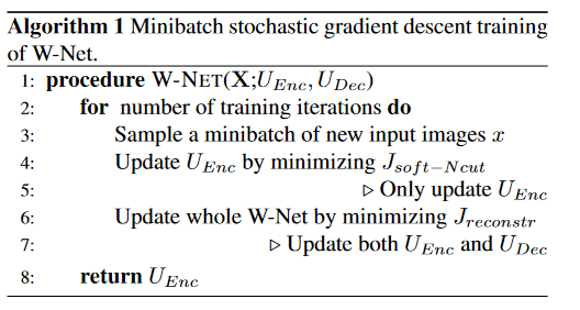
The algorithm to train the model is described as this in the paper:

The delivered function looks like this:

def train_op(model, optimizer, input, psi=0.5):
    enc = model(input, returns='enc')
    n_cut_loss=gradient_regularization(enc)*psi
    n_cut_loss.backward()
    optimizer.step()
    optimizer.zero_grad()
    dec = model(input, returns='dec')
    rec_loss=torch.mean(torch.pow(torch.pow(input, 2) + torch.pow(dec, 2), 0.5))*(1-psi)
    rec_loss.backward()
    optimizer.step()
    optimizer.zero_grad()
    return model

So we need to implemented the losses used in the paper, the reconstruction loss (rec_loss) is an easy one to implement. It looks like this:

So we need to minimize the distance between the original image X and the output of the decoder, given the segmentated output of the encoder.

def reconstruction_loss(x, x_prime):
    criterionIdt = torch.nn.MSELoss()
    rec_loss = criterionIdt(x_prime, x)
    return rec_loss

dec = model(input, returns='dec')
rec_loss=reconstruction_loss(input, dec)

This works because the model implements the decoder like this: dec=self.UDec(F.softmax(enc, 1)).

Add this loss to the train_op function

def train_op(model, optimizer, input, psi=0.5):
    enc = model(input, returns='enc')
    n_cut_loss=gradient_regularization(enc)*psi
    n_cut_loss.backward()
    optimizer.step()
    optimizer.zero_grad()
    dec = model(input, returns='dec')
    rec_loss=reconstruction_loss(input, dec)
    rec_loss.backward()
    optimizer.step()
    optimizer.zero_grad()
    return model

The Soft Normalized Cut Loss(soft_n_cut_loss) is a bit harder to implement. The function looks like this:

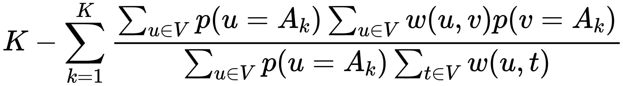
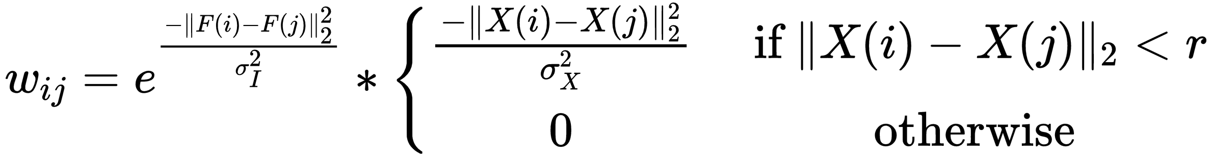
With w(u,v) being a weight between (u,v) and p being the probability value the encoder gives to an pixel belonging to group k, implementing w looks like this:

First thing we did was look at already existing implementations, of which we found two:

1. https://github.com/gr-b/W-Net-Pytorch², uses a matrix solution to compare all pixels with each other. Does not use the radius mentioned in the paper, although it is added as a argument. Some of the methods are also ported from a Tensorflow implementation, so the code has custom implementations for calls which already exist in the PyTorch API, like custom outer functions.
2. https://github.com/fkodom/wnet-unsupervised-image-segmentation³, which uses conv2d kernels to compare the pixels, which is much more efficient when working with large images. This implementation deviates from the paper by doing an pixel average, they mention this: “Small modifications have been made here for efficiency – specifically, we compute the pixel-wise weights relative to the class-wide average, rather than for every individual pixel.”

Instead of using these implementations, we decided to implement this loss ourselves and stay true to the paper.

Aproach 1: creating a weight matrix

Because we implemented this on our relatively low spec laptops we worked with 64x64 images while developing. So the matrix approach worked without giving memory issues, and was the first approach we did. The idea was similar to the first Github linked above, but the code is created on our own. The main idea was to create a weight matrix which compares all NxN pixels with each other. So this results in a weight matrix of size N*NxN*N, quite a big matrix but doable for image sizes of 64x64. To illustrate our approach we are going to use a 3x3 matrix, lets say we have this matrix.

tensor([[1., 2., 3.],
        [4., 5., 6.],
        [7., 8., 9.]])

We will flatten this image and expand it NxN times, creating this N*NxN*N matrix.

tensor([[1., 2., 3., 4., 5., 6., 7., 8., 9.],
        [1., 2., 3., 4., 5., 6., 7., 8., 9.],
        [1., 2., 3., 4., 5., 6., 7., 8., 9.],
        [1., 2., 3., 4., 5., 6., 7., 8., 9.],
        [1., 2., 3., 4., 5., 6., 7., 8., 9.],
        [1., 2., 3., 4., 5., 6., 7., 8., 9.],
        [1., 2., 3., 4., 5., 6., 7., 8., 9.],
        [1., 2., 3., 4., 5., 6., 7., 8., 9.],
        [1., 2., 3., 4., 5., 6., 7., 8., 9.]])

Now if we subtract from this matrix its own transponse we will get the difference between 2 values at position (i,j):

tensor([[ 0.,  1.,  2.,  3.,  4.,  5.,  6.,  7.,  8.],
        [-1.,  0.,  1.,  2.,  3.,  4.,  5.,  6.,  7.],
        [-2., -1.,  0.,  1.,  2.,  3.,  4.,  5.,  6.],
        [-3., -2., -1.,  0.,  1.,  2.,  3.,  4.,  5.],
        [-4., -3., -2., -1.,  0.,  1.,  2.,  3.,  4.],
        [-5., -4., -3., -2., -1.,  0.,  1.,  2.,  3.],
        [-6., -5., -4., -3., -2., -1.,  0.,  1.,  2.],
        [-7., -6., -5., -4., -3., -2., -1.,  0.,  1.],
        [-8., -7., -6., -5., -4., -3., -2., -1.,  0.]])

If we divide all these values by the given deviation parameter and put it on an expontial we will get the first part of the W matrix. The second part uses the radius, so that it only looks at pixels inside of the radius length.

To implement this radius constraint, we did the same thing again with the flattening and the expanding as above, but this time we created 2 matrices and used index locations as values. For example the matrix containing the X locations.

tensor([[0., 1., 2.],
        [0., 1., 2.],
        [0., 1., 2.]])

So after flattening, expanding and substracting it own transpose we have 2 matrices. One containing the distance on the X dimension and one for the Y dimension. If we add these distance we got the manhatten distance, but we want the euclidian one

Xij = (X_expand - X_expandT)
Yij = (Y_expand - Y_expandT)

sq_distance_matrix = torch.hypot(Xij, Yij)

So now we got the distances between pixels, we can set all distance to 0 if they are larger than the given radius using a mask. We first apply the mask to the sq_distance_matrix, divide this matrix and apply the exponential. After applying these transformations, the two matrices are multiplied to create the final weight matrix

mask = sq_distance_matrix.le(radius)

C = torch.exp(torch.div(-1*(sq_distance_matrix **2), ox**2))
W_X = torch.mul(mask, C)

weights = torch.mul(W_F, W_X)

Now we can use this weight matrix and the results of the encoder to calculate the soft_n_cut_loss, but the paper mentioned that they trained on images of size 224x224. Using the weight matrix method on images of this size result in multiple matrices of size 50176x50176.

Aproach 2: custom sliding window

The second idea is based on the local computation involving the radius. The weights are 0 for pixels that are farther away than the radius. So the calculations needed could be contained to a window of size radius*2 + 1, the plus 1 so that the kernel has an uneven size and has a good center.

Lets consider the following image:

tensor([[0.3337, 0.1697, 0.4311, 0.5673, 0.5980],
        [0.2870, 0.0539, 0.2289, 0.3007, 0.6262],
        [0.0553, 0.8031, 0.9282, 0.0542, 0.3415],
        [0.7486, 0.5111, 0.2467, 0.0990, 0.6030],
        [0.2950, 0.8395, 0.8924, 0.7440, 0.5326]])

We need to do this window operation on every pixel on this image, so we need to add padding to this image the same size as the radius. Doing this gives us the following first and second window for radius = 1:

tensor([[0, 0, 0],
        [0, 0.3337,  0.1697],
        [0, 0.2870, 0.0539]])

tensor([[0, 0, 0],
        [0.3337, 0.1697, 0.4311],
        [0.2870, 0.0539, 0.2289]])

We have no definite answers on what values are best to use for the padding. The assumption we have right now is that it does not matter, but we did not have enough time to test and prove this assumption.

For each of these windows we create two seperate windows, one containing only the center values(c_values_window) and the second one consisting of relative euclidian distances(distance_weights_windows).

The c_values_window window is used to calculate the distance for each element compared to the center in the original window, this is done by subtraction.

For the location distance we can create a window filled with relative distances. And remove the values farther away than the radius since the kernel will be a square.

The 2 matrices, c_values_window and distance_weights_windows, will look like this. The second matrix will have the corners set to 0 since this kernel is created with a radius of 1

tensor([[0.3337, 0.3337, 0.3337],
        [0.3337, 0.3337, 0.3337],
        [0.3337, 0.3337, 0.3337]])

tensor([[1.43 , 1, 1.43],
        [1    , 0, 1   ],
        [1.43 , 1, 1.43]])

Now we have an image split up in X amount of pixel value windows, depending on the image size and the radius used. We can similary do the same for the output of the encoder. Create the same X amount of windows.

We can sum all these windows and create a matrix with the same shape as the original image. Where each (i,j) location contains weights summed up for that (i,j) centered window. Now we just do an element wise multiplication between the layer of the encoder output and the newly generated matrix. This method works great, we can even do this batchwise across multiple images and we do this very efficiently, and this stays true to the paper.

Post-processing

Since the output of the encoder shows the hidden representation, but is still rough. The postprocessing algorithm can be found in the image under Algorithm 2. We apply postprocessing to the encoder output. A fully conditional random field is applied to smooth the encoder output and provide a more simple segmentation with larger segments. Furthermore, we see that the probability boundary is computed with the contour2ucm method. We have not implemented this postprocessing step as was discussed with the supervisor for this paper.

Results

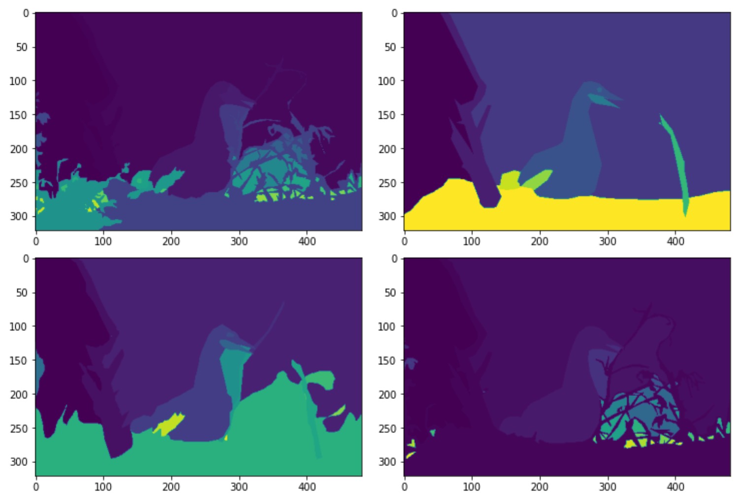
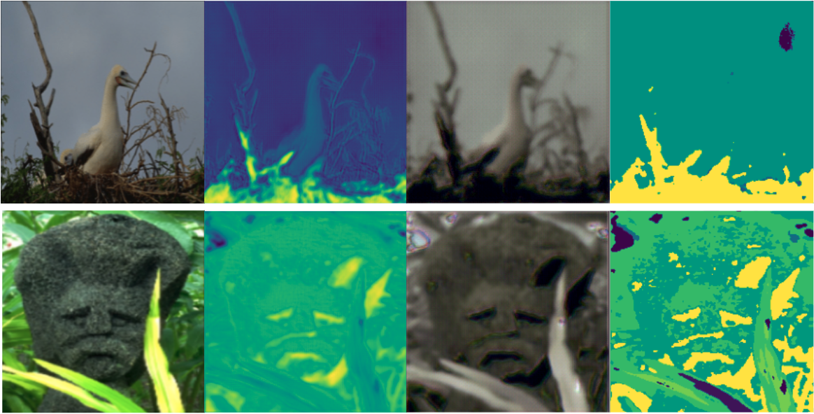
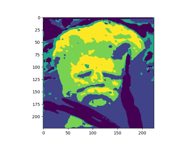
The models were trained on a Google Cloud compute engine running in zone us-west-1b. The machine was initialized with CUDA support and running PyTorch 1.8. The specifications of the machine state the N1 high-memory 2 vCPU’s with 13GB RAM, and it was additionally beefed up with a NVIDIA Tesla K80 sporting 24GB RAM. The following images were with a small dataset of 10 images and 100 epochs. The squeeze layer is of size 22 and dropout is set to 0.15. Left to right: Input image, Encoder output, Decoder reconstruction, CRF smoothed encoding.

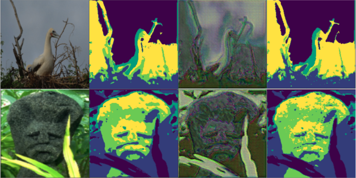
We also trained our model locally on 1 image, we did this for 300 epochs with a learning_rate=0.003. Left to right: Input image, Encoder output, Decoder reconstruction, CRF smoothed encoding.

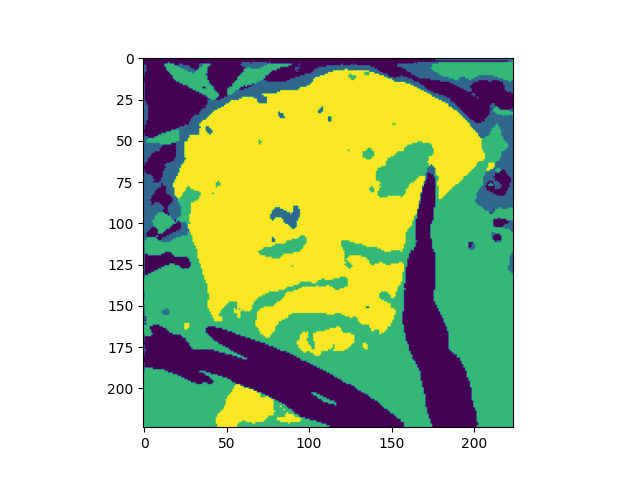
Below are the results for squeeze=4 and squeeze=6.

Benchmarking

The postprocessed output of the encoder will be benchmarked against the groundtruth of the BSD300 and BSD500 dataset. The benchmarks were only mentioned and not thoroughly explained in the paper. There was also additional rescaling involved, the output of the Encoder had a square aspect ratio, whereas the Berkeley Segmentation Dataset featured either landscape, or portrait images. We use opencv for resizing the segmentations with the following procedure:

segment_truth_ods = cv2.resize(segment_truth, dsize=(224, 224), interpolation=cv2.INTER_NEAREST)

We resize the image with nearest neighbor resampling, in this way we retain having similar labelling as before resizing. The benchmarks will include Segmentation Covering, Variation of information and Probabilistic Rand Index, these are thoroughly explained in the paper by Arbelaez et al. ⁴ which is cited in the paper, however an implementation of them was not found in the Github repository. There is benchmarking code available on the BSD website, but this meant the segmentations had to be reencoded into matlab. Since the benchmarking is a large part of the reproduction we decided to try implementing it ourselves. We will go over the implementation in the following sections and a full notebook can be found in the repository. We have some doubts about the correctness of these benchmarks, if one needs to be sure, they can use the benchmarking code from the Berkeley Segmentation Dataset, however the output of the segmentation need to be converted to .mat files first.

Segmentation Covering

To calculate the segmentation overlap, we first need the formula to calculate the overlap of two segments. This is basically intersection over union.

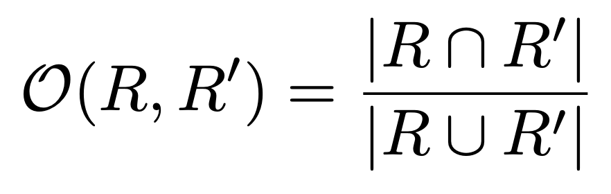
With this overlap, we calculate the segmentation covering with the following forumula:

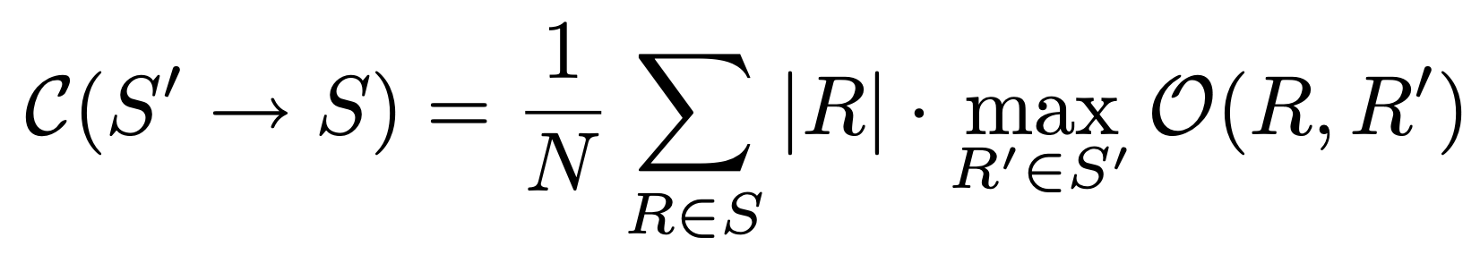
Where N is the number of segments, R is a segment in segmentation S and |R| the size of this segmentation. The formula looks for the maximum segmentation covering and sums this for the final result, dividing over the number of pixels.

The implementation in Python is as follows, Where the overlap is calculated by:

def calculate_overlap(r1, r2):
    # intersection
    a = np.count_nonzero(r1 * r2)
    # union
    b = np.count_nonzero(r1 + r2)
    
    return a/b

And then the full segmentation covering:

def calculate_segmentation_covering(segmentation1, segmentation2):
    assert segmentation1.shape == segmentation2.shape, "segmentations should be same size"
    
    N = segmentation1.shape[0] * segmentation1.shape[1]
    
    maxcoverings_sum = 0
    
    # Sum over regions
    for label1 in np.unique(segmentation1):
        # region is where the segmentation has a specific label
        region1 = (segmentation1 == label1).astype(int) 
        # |R| is the size of nonzero elements as this the region size
        len_r = np.count_nonzero(region1) 
        max_overlap = 0
        # Calculate max overlap 
        for label2 in np.unique(segmentation2):
            # region is where the segmentation has a specific label
            region2 = (segmentation2 == label2).astype(int)
            # Calculate overlap
            overlap = calculate_overlap(region1, region2)
            max_overlap = max(max_overlap, overlap)
        
        maxcoverings_sum += (len_r * max_overlap)
        
    return (1 / N) * maxcoverings_sum

Probabilistic Rand Index

The probabilistic rand index is an extension of the rand index. The rand index is a measure of the similarity between segmentations on a pixel level. It looks at which pixels are assigned to which segment and if these segments have the same pixel assigned. The probabilistic rand index also extends on this by checking the probability of having the same label.

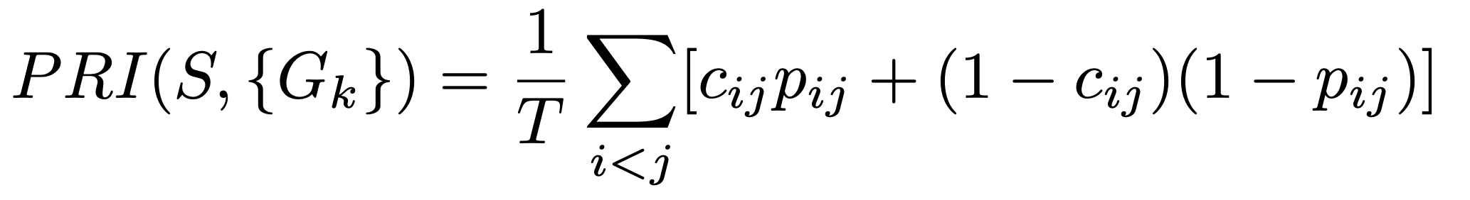
Where S is a segmentation and {Gk} the ground truth segmentations. T is the total number of elements and c_ij is the event that pixel i and pixel j are in the same segmentation. We looked at both segmentations and checked if they have the same label for this. the probability p_ij is the probability of this pixel being the same. We calculated this as the probability of a pixel having a certain label in the set of all labels in the segmentations and multiplying this probability from both segments. We are not sure if this is the right way to do it, the linked paper which explained these different benchmarks also did not go in-depth on this. Multiple searches on the internet only provide the adjusted rand index and the normal rand index.

While this was the hardest benchmark to comprehend, we attempted to implement it. Since each pixel pair is considered, there is downscaling involved as computing this on large scale images would be insanely computationally intensive. This is how we implemented it in Python, although we have some doubts on whether this is correct.

import math

def calculate_probabilistic_rand_index(segmentation1, segmentation2):
    assert segmentation1.shape == segmentation2.shape, "segmentations should be same size"
    
    a1 = math.floor(segmentation1.shape[0]/10)
    a2 = math.floor(segmentation1.shape[1]/10)
    
    segmentation1 = cv2.resize(segmentation1, dsize=(a1, a2), interpolation=cv2.INTER_NEAREST)
    segmentation2 = cv2.resize(segmentation2, dsize=(a1, a2), interpolation=cv2.INTER_NEAREST)
    
    segmentation1_flat = segmentation1.flatten()
    segmentation2_flat = segmentation2.flatten()
    
    n = len(segmentation1_flat)
    m = len(segmentation2_flat)
    
    T = n * m
    
    # first calculate pixel probabilities
    prob_segment1 = {}
    for label in np.unique(segmentation1):
        prob_segment1[label] = np.count_nonzero(segmentation1 == label) / n
    
    prob_segment2 = {}
    for label in np.unique(segmentation2):
        prob_segment2[label] = np.count_nonzero(segmentation2 == label) / m
        
    rand_index_sum = 0 
    
    # Then perform main loop
    for i in range(n):
        for j in range(i,m):
            pixeli = segmentation1_flat[i]
            pixelj = segmentation2_flat[j]
            # event that pixels i and j have the same label 
            c_ij = pixeli == pixelj
            # probability that pixels i and j have the same label
            p_ij = prob_segment1[pixeli] * prob_segment2[pixelj]
            rand_index_sum += c_ij * p_ij + (1 - c_ij) * (1 - p_ij)
    
    
    return (1 / T) * rand_index_sum

Variation of Information

Variation of information looks at the entropy of both segmentations and the mutual information between them. This is given by the formula.

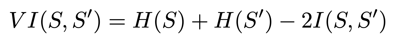
We implemented this in python using Scikit-learn and Scikit-image functions:

import skimage.measure
import sklearn.metrics

def calculate_variation_of_information(segmentation1, segmentation2):
    assert segmentation1.shape == segmentation2.shape, "segmentations should be same size"
    
    ret = skimage.measure.shannon_entropy(segmentation1)
    ret += skimage.measure.shannon_entropy(segmentation2)
    ret -= 2 * sklearn.metrics.mutual_info_score(segmentation1.flatten(), segmentation2.flatten())
    return ret

Benchmarking Results

We show the results of a model trained for a model with 400 epochs, 40 batches and a batch size of 5. On the BSD500 test dataset, comparing to the W-Net model from the paper. For SC and PRI, higher scores are better. for VI, a lower score is better.

Method	SC		PRI		VI
	ODS	OIS	ODS	OIS	ODS	OIS
WNet (paper)	0.57	0.62	0.81	0.84	1.76	1.60
WNet (ours)	0.44	0.44	0.41	0.41	2.44	2.43

We see that our model has worse segmentation covering than the model in the paper, with no differences between optimal data set scale and optimal image scale. The probabilistic rand index is much much lower than in the paper, however we have trained on a downscaled ground truth and image size to preserve computational time and as mentioned before we are sceptic about our implementation of the PRI. Variation of information is much worse than the model in the paper. We have seen better results when running on a single image and comparing that with the ground truth.

Reproduction Discussion

Both of us had around 100 dollars to spend on google cloud for training our models. Since we were novice in cloud computing, of course some of the budget was wasted on models that resulted in nothing useful. But for the most we found that training a model with 400 epochs, 40 batches and a batch size of 5 took around 10 hours to train and cost around 8-10 dollars. Given the fact that the original authors trained the model for 50000 epochs on the full 12000 image dataset, achieving the same result is infeasible as it would never fit in our budget and time for the project. That said, one could cut costs by having their own dedicated hardware, with the expenses we have made you can buy a nice GPU to train your model on (assuming you can get a GPU at MSRP during this semiconductor shortage).

Conclusion

We have demonstrated a reproduction of the paper “W-net: A Deep Model for Fully Unsupervised Image Segmentation.”. We have explained the dataset, the model, losses and postprocessing. Furthermore, we have demonstrated our preliminary results and explained our benchmarking approach of the project. For us, we have gotten the experience of reproducing a paper with incomplete code. We see that even when fixing the codebase to the specifications of the paper, being able to train and test the implemented models could be infeasible for a normal computer science/artificial intelligence student. We believe the code, that we have implemented right now, is complete and true to the paper, but we did not get the chance to run it in the same way as the paper.

References

1. T. (2018, October 17). taoroalin/WNet. GitHub. https://github.com/taoroalin/WNet ↩

2. G. (2019, November 26). gr-b/W-Net-Pytorch. GitHub. https://github.com/gr-b/W-Net-Pytorch ↩

3. F. (2019a, June 13). fkodom/wnet-unsupervised-image-segmentation. GitHub. https://github.com/fkodom/wnet-unsupervised-image-segmentation ↩

4. Arbeláez, P., Maire, M., Fowlkes, C., & Malik, J. (2011). Contour Detection and Hierarchical Image Segmentation. IEEE Transactions on Pattern Analysis and Machine Intelligence, 33(5), 898–916. https://doi.org/10.1109/tpami.2010.161 ↩